Quantum computing is among the most exciting technologies under active development today. Since the discovery of Shor’s algorithm, the prospect of addressing important, classically-hard problems has drawn increasing interest from industry and academia, while intriguing many more in the general public. Rapid, ongoing progress in pursuit of fault-tolerant quantum computers has propelled the field into the so-called noisy intermediate-scale quantum era, where state-of-the-art applications employ hybrid algorithms, using both quantum and classical resources.

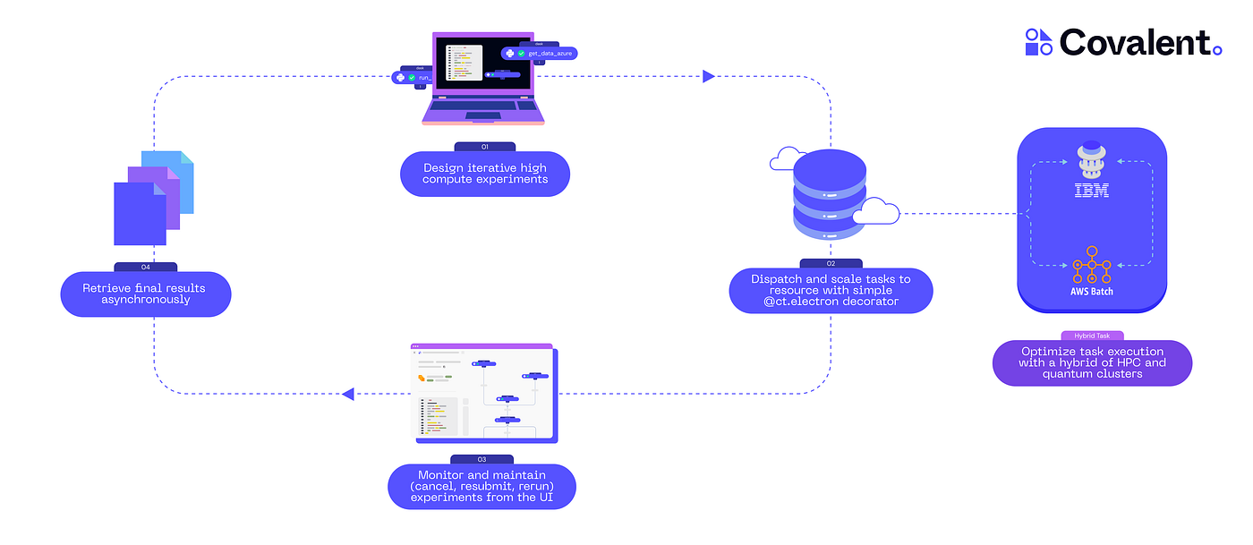
With quantum processing units (QPUs) becoming readily available over the cloud, the modern computing landscape has become all the more diverse. Users can rely on services like IBM’s Qiskit Runtime to access real quantum hardware, while benefiting from free tools like Qiskit to implement their quantum programs. In the context of hybrid applications, many users additionally rely on other cloud services, such as AWS, GCP, or Azure, to execute intensive classical computations inside a given algorithm. To alleviate the challenges inherent to this heterogeneous approach, this post introduces Covalent — an open-source orchestration tool for running distributed workflows across various platforms.

Covalent simplifies cloud computing for quantum and classical developers by providing a high-level Python interface and an interactive UI for managing complicated workflows. We will showcase these features here in a tutorial-style introduction, where we implement a hybrid neural network using IBM Quantum together with AWSBatch.

Let’s start with a brief overview of the Covalent SDK.

Covalent Basics

Getting Started

Covalent can be installed by simply running

pip install covalent

from the command line. We also provide a Quick Start guide in our documentation for new users. If you’re interested in more technical details, or wish to contribute to the project, please see the Covalent page on GitHub.

Covalent SDK

The Covalent SDK is a simple-to-use Python library consisting of three main components that provide granular control of individual workflow tasks:

1. the “electron” decorator (@ct.electron) – designates a task
2. the “lattice” decorator (@ct.lattice) – defines a workflow
3. various “executors” (ex. AWSBatchExecutor) – define task execution

In Covalent, an “electron” is a single, dispatchable task created by using the @ct.electron decorator on top of any Python function. The following example shows a simple electron:

import covalent as ct

@ct.electron
def task(x):
    return x + 1

Similarly, a “lattice” is a workflow that contains one or more electrons, and is created using the @ct.lattice decorator. Below, we have a lattice that calls two electrons (task1 and task2):

@ct.electron
def task1(x):
    return x + 1

@ct.electron
def task2(x):
    return x * 2

@ct.lattice
def workflow(x):
    y = task1(x)
    z = task2(y)
    return z

Finally, the “executor” component is what makes Covalent truly heterogeneous. It serves as an abstraction layer for offloading tasks to various platforms including cloud services, on-premises hardware, QPUs, GPUs, and more. We can run any electron on a resource of our choosing by simply passing an instance of that executor to the given electron:

# to run electrons on AWSBatch
batch_executor = ct.executors.AWSBatchExecutor(
    batch_queue = "test-queue",
    vcpu = 8,
    memory = 32,
    num_gpus = 1,
    time_limit = 36000 
)

@ct.electron(executor=batch_executor)
def task(x):
    return x + 1

After creating electrons and lattices, we dispatch the lattice and asynchronously retrieve the final result using Covalent’s dispatch() and get_result() functions, respectively:

# Dispatch the workflow lattice
dispatch_id = ct.dispatch(workflow)(x=3)

# Retrieve the result of the lattice computation
result = ct.get_result(dispatch_id=dispatch_id, wait=True)

# Print the result
print("Result: ", result.result)

Beyond the SDK, Covalent aids workflow management with features like metadata collection, a rich UI, and easy scaling across local, distributed, hybrid, or multi-cloud configurations.

Workflow Preview

To help cement the ideas above, here’s a rough (and abridged) outline of the final experimental code that we’ll develop in this post.

# quantum-classical neural network that uses
# IBM Quantum for QPUs, AWS for classical compute
import os
import matplotlib, qiskit, qiskit_ibm_runtime, torch

TOKEN = os.environ["IBM_QUANTUM_TOKEN"]

@ct.electron(executor=batch_executor)
def train_model(backend_name, n_shots, n_epochs, **kw):
    # runs on AWS
    # access IBM Quantum QPU's via `Estimator` from Qiskit Runtime
    ...

@ct.electron
def plot_predictions(model_state):
    # runs locally
    # use simulator to evaluate model via `Estimator` from Qiskit
    ...
  
@ct.lattice
def hybrid_workflow(backend_name, n_shots, n_epochs, **kw):
    # a simple two-step workflow:
  
    # train the neural network
    result = train_model(backend_name, n_shots, n_epochs, **kw)
  
    # use it to make predictions
    plot_predictions(result)
    return result
  

# dispatch
ct.dispatch(hybrid_workflow)("ibm_nairobi", 100, 5, batch_size=16)

We have omitted implementation details here to better emphasize Covalent’s scope in the present example. Details aside, one can think of the above as a regular Python script, plus a handful of quick changes (via the Covalent SDK) that make it cloud-ready.

Implementing the Quantum Layer

We adapt an example from Qiskit Textbook, which uses Qiskit and PyTorch to implement a trainable quantum layer inside a classical neural network (n.n.). An instructive figure from Qiskit Textbook, which illustrates a basic architecture for quantum-classical n.n.s, is reproduced below.

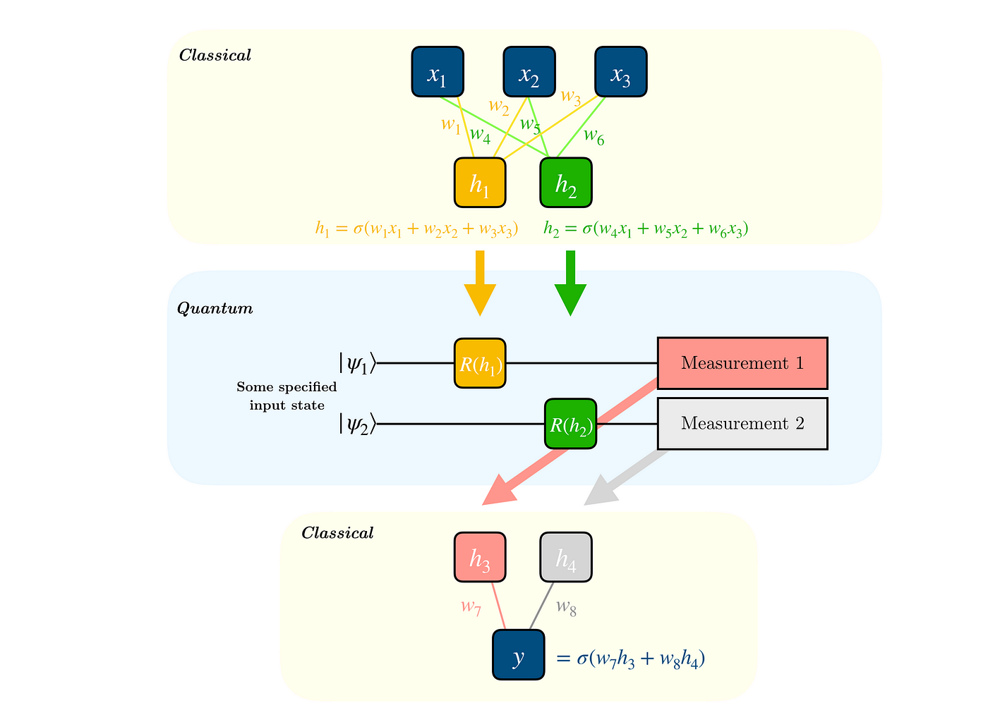
Building upon the textbook example, we modify the original Qiskit code to utilize IBM QPUs via the Estimator primitive from Qiskit Runtime. This requires some changes to the first abstraction layer, which encapsulates all the “quantum” parts of our program. The relevant changes are reflected in the run method of the class below.

import torch
from qiskit import QuantumCircuit, QuantumRegister
from qiskit.circuit import Parameter
from qiskit.quantum_info import SparsePauliOp
from qiskit_ibm_runtime import Estimator


class MyQuantumCircuit:
    """simple interface for running parametric quantum circuits"""
    def __init__(self, n_qubits: int, shift: float, estimator: Estimator):
        self.n_qubits = n_qubits
        self.shift = shift
        self.estimator = estimator
        self._init_circuit_and_observable()

    def run(self, inputs: torch.Tensor) -> torch.Tensor:
    """access IBM QPU's using Qiskit Runtime"""
        parameter_values = inputs.tolist()
        circuits = [self.circuit] * len(parameter_values)
        observables = [self.obs] * len(parameter_values)

        job = self.estimator.run(  # runs on an IBM Quantum QPU
            circuits=circuits,
            observables=observables,
            parameter_values=parameter_values
        )
        exps = job.result().values
        return torch.tensor(exps).unsqueeze(dim=0).T

    def _init_circuit_and_observable(self) -> None:
        qr = QuantumRegister(size=self.n_qubits)
        self.circuit = QuantumCircuit(qr)
        self.circuit.barrier()
        self.circuit.h(range(self.n_qubits))
        self.thetas = []
        for i in range(self.n_qubits):
            theta = Parameter(f"theta{i}")
            self.circuit.ry(theta, i)
            self.thetas.append(theta)

        self.circuit.assign_parameters({theta: 0.0 for theta in self.thetas})
        self.obs = SparsePauliOp("Z" * self.n_qubits)

As in the original, we also subclass torch.autograd.Function and override its forward and backward methods to map inputs to quantum circuit parameters and to calculate gradients using the parameter-shift rule, respectively. Here, both the forward and backward passes rely on the run method of a MyQuantumCircuit instance (the variable qc).

class QuantumFunction(torch.autograd.Function):
    """custom autograd function that uses a quantum circuit"""
    @staticmethod
    def forward(ctx, batch_inputs: torch.Tensor, qc: MyQuantumCircuit):
        """forward pass computation"""
        ctx.save_for_backward(batch_inputs)
        ctx.qc = qc
        return qc.run(batch_inputs)

    @staticmethod
    def backward(context, grad_output: torch.Tensor):
        batch_inputs = context.saved_tensors[0]
        qc = context.qc
        shifted_inputs_r = torch.empty(batch_inputs.shape)
        shifted_inputs_l = torch.empty(batch_inputs.shape)

        # loop over each input in the batch
        for i, _input in enumerate(batch_inputs):
            # loop entries in each input
            for j in range(len(_input)):
                # compute parameters for parameter shift rule
                d = torch.zeros(_input.shape)
                d[j] = qc.shift
                shifted_inputs_r[i, j] = _input + d
                shifted_inputs_l[i, j] = _input - d

        # run gradients in batches
        exps_r = qc.run(shifted_inputs_r)
        exps_l = qc.run(shifted_inputs_l)
        return (exps_r - exps_l).float() * grad_output.float(), None, None

Creating the Hybrid Neural Network

Instead of classifying 0’s and 1’s from MNIST dataset, our n.n. will classify images of dogs and cats from this public dataset. Having laid the groundwork in the previous section, we can build a basic sequential n.n. for the task at hand by appending a quantum layer (with n_qubits=1) to a base model that uses the ResNet architecture [1]:

from qiskit_ibm_runtime import IBMBackend, Options
from torchvision.models import resnet34

def get_model(
    n_qubits: int,
    backend: IBMBackend,
    options: Options,
) -> torch.nn.Sequential:

    # initialize an estimator
    estimator = Estimator(session=backend, options=options)

    # --- CREATE HYBRID MODEL --- #
    resnet_model = resnet34(weights="ResNet34_Weights.DEFAULT")
    for params in resnet_model.parameters():
        params.requires_grad_ = False
    
    resnet_model.fc = torch.nn.Linear(resnet_model.fc.in_features, n_qubits)
    model = torch.nn.Sequential(
        resnet_model,
        QuantumLayer(n_qubits, estimator),
    )
    model.to("cuda" if torch.cuda.is_available() else "cpu")
    
    return model

While this network does not offer any real advantage, it serves as an illustrative example of a hybrid n.n. that uses real quantum hardware. The steps outlined here and in the preceding sections are easily adaptable to less trivial problems. However, for demonstration purposes, we’ll keep things light.

Notice that get_model is not an electron (nor does it need to be) because it is not explicitly called inside the lattice (i.e., the decorated hybrid_workflow function). We can nonetheless use get_model freely inside train_model, which is an electron and will run on AWS.

Finalizing the Code

The n.n. returned by get_model is subsequently trained using a standard PyTorch training loop over 1 epoch, with size-16 batches of sample data. This is done inside the train_model function (electron), which calls get_model as well as another function that prepares the input data. In the interest of brevity, we omit the implementation here and refer the reader to the final production code for further details. When the workflow is dispatched and the train_model task runs on AWS, it will initialize an Estimator instance from Qiskit Runtime in the usual way and use it to submit jobs to IBM Quantum, whenever the QuantumLayer is applied in the network.

The only other electron, plot_predictions, will use the Estimator class from qiskit.primitives to make predictions with the trained model on a local simulator and visualize the results. This electron will run on the user’s machine, using the default Dask executor.

Execute on AWS using Covalent: Streamlining Hybrid Quantum Workflows

Let’s return to the “Workflow Preview” section and flesh out some of the remaining details.

Unless the user has configured Covalent and AWSBatch to use a specific container when executing train_model, we’ll need to specify some dependencies to prepare the execution environment:

DEPS_PIP = [
    "torch==2.0.0",
    "torchvision==0.15.1",
    "qiskit==0.42.0",
    "qiskit_ibm_runtime==0.9.1"
]

To ensure easy access to the input data, which we’ve reduced it to a modest 1% of the original dataset and uploaded it to an Amazon S3 bucket. Covalent’s file transfer mechanism allows us to download these files automatically whenever executing the train_model electron on a freshly allocated compute instance.

# downloads file from S3 bucket to remote filesystem
DATA_FT = ct.fs.FileTransfer(
    from_file="s3://my-s3-bucket/dogs_vs_cats_0.01.zip",
    to_file="dogs_vs_cats_0.01.zip",
    strategy=ct.fs_strategies.S3()
)

We then simply modify the @ct.electron decorator to associate the above file transfer and dependencies with the train_model electron:

@ct.electron(executor=batch_executor, deps_pip=DEPS_PIP, files=[DATA_FT])
def train_model(backend_name, n_shots, n_epochs, files=None, **kw):
    # runs on AWS
    # access IBM Quantum QPU's via `Estimator` from Qiskit Runtime
    ...

The other, locally-executed plot_predictions electron needs no further modification.

To dispatch the heterogenous workflow, we simply run

dispatch_id = ct.dispatch(hybrid_workflow)("ibm_nairobi", 100, 1, batch_size=16)
print("dispatch_id:", dispatch_id)

result = ct.get_result(dispatch_id=dispatch_id, wait=True)
print(result.result)

If the Covalent server is running on the user’s machine, then navigating to http://localhost:48008 in a browser will display the Covalent UI. Here, among execution parameters and other metadata, we’ll find a transport graph that visualizes interdependencies between electrons comprising our hybrid workflow.

Results

Training over the reduced, 400-datapoint training set requires 25 iterations per epoch, for a batch size of 16. Plotting the loss over a single epoch produces a familiar graph below.

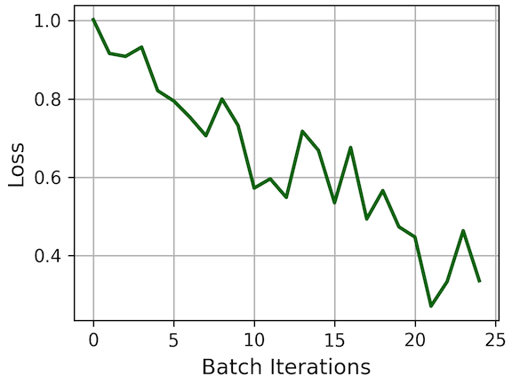
In this example, the loss was computed between 16 targets and 16 predictions, both as vectors of 1’s and -1’s, indicating “dog” and “cat”, respectively. Altogether, the 25 batch iterations involve 75 calls to IBM Quantum, each submitting a job that runs 16 circuits (one for each datum in the batch). Note that the number of jobs is three times the number of batch iterations, because we use parameter shifts (2 extra jobs per circuit parameter) to calculate the gradients of the quantum circuit — these are also batched into 16 circuits each for the left- and right-shifted inputs.

It bears repeating that the hybrid workflow developed herein serves a mostly demonstrative purpose. To keep the example accessible for free-tier users, we employed a pre-trained classical ResNet that does most of the heavy lifting. The combined model nonetheless benefits from a quick training run to tune the parameters for the appended quantum layer.

The output of the plot_predictions electron is the figure below. The predicted label is determined from the sign of the value in parentheses, under each image.

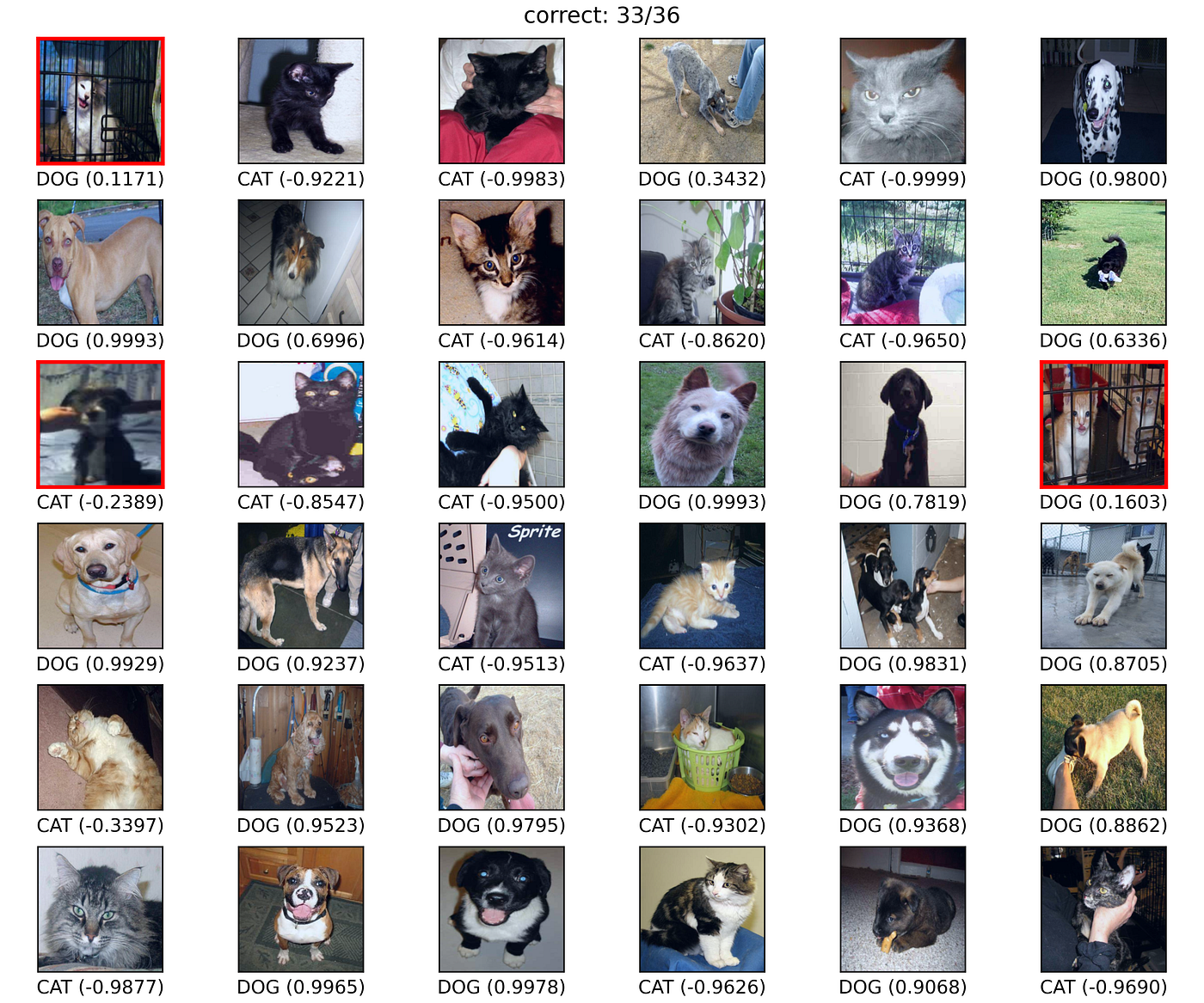
Notice that the output is near 0 for all incorrectly-predicted labels (images outlined red). This is encouraging as it implies that the model is unsure, rather than confidently wrong. By contrast, the majority of correctly-predicted labels correspond to outputs near 1 or -1.

Expanding Scope

Beyond the minimal example, a full-scale machine learning workflow should include hyperparameter tuning to select non-learnable parameters. With Covalent, we can easily adapt the existing workflow to perform a grid search using multiple concurrent runs.

One way to do this is to introduce a simple for loop in the lattice function. For example, with only a small modification, we have:

@ct.lattice
def hybrid_workflow(backend_name, n_shots, n_epochs, batch_sizes):
    results = []
    # --> NEW: loop over several batch sizes <--
    for batch_size in batch_sizes:
  
        # train the neural network using given batch size
        result = train_model(backend_name, n_shots, n_epochs, batch_size=batch_size)
    
        # use it to make predictions
        plot_predictions(result)
        results.append(result)
    
    return results
  
# dispatch concurrent grid search
ct.dispatch(hybrid_workflow)("ibm_nairobi", 100, 5, batch_sizes=[16, 24, 32])

Covalent will recognize independent tasks in the workflow and start every task that doest not depend on outputs for other tasks. We can see this most clearly in the Covalent UI.

For more complicated workflows, Covalent also allows converting lattices to sublattices, which lets uses deploy smaller workflows as a self-contained units inside another lattice.

Conclusion

In this blog post, we adapted a tutorial from Qiskit Textbook, using Qiskit and PyTorch to create a quantum layer inside a classical neural network. This original example was developed further to (1) use real QPUs via Qiskit Runtime and (2) classify colour images of dogs versus cats.

This culminated in a hybrid workflow that we made cloud-ready with just a few lines of code, by utilizing the Covalent SDK. Using a pre-trained ResNet [1] as a base model allowed for a brief but effective training run, making a reasonable 75 job submissions to IBM Quantum.

In general, Covalent can handle much more complex workflows (see the deep learning tutorial, for example). Because task interdependencies are determined automatically, expanding an existing workflow is as easy as modifying the logic of the lattice function (hybrid_workflow in this case); adding loops, conditional statements, or writing more electrons. Crucially, the user can deploy a given task on a different resource by simply introducing a different executor. This means that we require minimal changes to run the quantum-classical neural network on say, a SLURM cluster instead of an EC2 instance via AWSBatch.

For further clarity, we’ve summarized some key features of Covalent below:

1. Integrating heterogenous resources: Covalent seamlessly interconnects resources like AWS, GCP, and Azure, as well as local or on-premises hardware. We used Covalent to offload a compute-intensive classical task, train_model, which also relies on IBM quantum hardware, to an EC2 instance on AWS. Meanwhile, we ran the lighter task in our workflow, plot_predictions, on the local machine.
2. Automatic management of task interdependencies: Covalent automatically determines the interdependencies between tasks, thereby simplifying the development process. We saw how Covalent intelligently handles dependencies between the train_model and plot_predictions electrons, particularly when expanding the scope to include a hyperparameter sweep.
3. Flexible workflow expansion: Expanding an existing workflow is as simple as modifying the lattice function’s logic. Users can easily add loops, conditional statements, or write new electrons to accommodate their needs.
4. Resource adaptability: Covalent lets you deploy different tasks on different resources with minimal effort. By introducing other executors, users can switch from an EC2 instance via AWSBatch to a SLURM cluster (or other resources) without any changes to experimental logic. For a full list of support platforms, please see the list of Covalent’s executor plugins.

Check out the Quick Start guide to get started with Covalent today!